Point clouds

We cover in this tutorial how to solve OT problems between two pointclouds by instantiating a PointCloud geometry.

import sys

if "google.colab" in sys.modules:
    !pip install -q git+https://github.com/ott-jax/ott@main

from IPython import display

import jax
import jax.numpy as jnp

import matplotlib.pyplot as plt

import ott
from ott.geometry import costs, pointcloud
from ott.problems.linear import linear_problem
from ott.solvers.linear import sinkhorn

Creates a PointCloud geometry

def create_points(rng, n, m, d):
    rngs = jax.random.split(rng, 3)
    x = jax.random.normal(rngs[0], (n, d)) + 1
    y = jax.random.uniform(rngs[1], (m, d))
    return x, y


rng = jax.random.PRNGKey(0)
n, m, d = 13, 17, 2
x, y = create_points(rng, n=n, m=m, d=d)
geom = pointcloud.PointCloud(x, y)

Computes the regularized optimal transport

To compute the transport matrix between the two point clouds, one defines first a PointCloud geometry

A PointCloud geometry holds two arrays of vectors (supporting the two measures of interest), along with a cost function (a CostFn object, set by default to SqEuclidean) and, possibly, an Epsilon regularization parameter.

This geometry object defines a LinearProblem object, which contains all the data needed to instantiate a linear OT problem (see the Gromov-Wasserstein tutorial for quadratic OT problems).

We can then call a Sinkhorn solver to solve that problem, and compute the OT between these points clouds. Note that all weights are assumed to be uniform in this notebook, but non-uniform weights can be passed as a=..., b=... arguments when defining the LinearProblem below.

# Define a linear problem with that cost structure.
ot_prob = linear_problem.LinearProblem(geom)
# Create a Sinkhorn solver
solver = sinkhorn.Sinkhorn()
# Solve OT problem
ot = solver(ot_prob)
# The out object contains many things, among which the regularized OT cost
print(
    " Sinkhorn has converged: ",
    ot.converged,
    "\n",
    "Error upon last iteration: ",
    ot.errors[(ot.errors > -1)][-1],
    "\n",
    "Sinkhorn required ",
    jnp.sum(ot.errors > -1),
    " iterations to converge. \n",
    "Entropy regularized OT cost: ",
    ot.reg_ot_cost,
    "\n",
    "OT cost (without entropy): ",
    jnp.sum(ot.matrix * ot.geom.cost_matrix),
)

 Sinkhorn has converged:  True 
 Error upon last iteration:  0.00068787485 
 Sinkhorn required  6  iterations to converge. 
 Entropy regularized OT cost:  1.4432423 
 OT cost (without entropy):  1.2848572

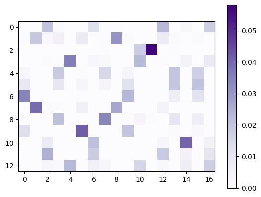
The ot output object contains several callables and properties, notably a simple way to instantiate, if needed, the OT matrix.

# you can instantiate the OT matrix
P = ot.matrix
plt.imshow(P, cmap="Purples")
plt.colorbar();

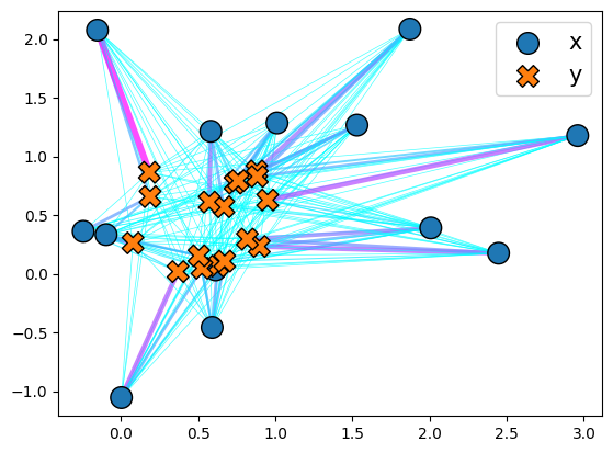
You can also instantiate a plott object to help visualize the transport in 2D.

plott = ott.tools.plot.Plot()
_ = plott(ot)

OT Gradient Flows

OTT returns quantities that are differentiable. In the following example, we leverage the gradients to move \(n\) points in a way that minimizes the overall regularized OT cost, given a ground cost function.

We start by defining a minimal optimization loop, that does fixed-length gradient descent, and records various ot objects along the way for plotting. By choosing various cost functions, we can then plot different types of gradient flows for the point cloud in \(x\).

def optimize(
    x: jnp.ndarray,
    y: jnp.ndarray,
    num_iter: int = 300,
    dump_every: int = 5,
    learning_rate: float = 0.2,
    **kwargs,  # passed to the pointcloud.PointCloud geometry
):
    # Wrapper function that returns OT cost and OT output given a geometry.
    def reg_ot_cost(geom):
        out = sinkhorn.Sinkhorn()(linear_problem.LinearProblem(geom))
        return out.reg_ot_cost, out

    # Apply jax.value_and_grad operator. Note that we make explicit that
    # we only wish to compute gradients w.r.t the first output,
    # using the has_aux flag. We also jit that function.
    reg_ot_cost_vg = jax.jit(jax.value_and_grad(reg_ot_cost, has_aux=True))

    # Run a naive, fixed stepsize, gradient descent on locations `x`.
    ots = []
    for i in range(0, num_iter + 1):
        geom = pointcloud.PointCloud(x, y, **kwargs)
        (reg_ot_cost, ot), geom_g = reg_ot_cost_vg(geom)
        assert ot.converged
        x = x - geom_g.x * learning_rate
        if i % dump_every == 0:
            ots.append(ot)
    return ots

# Helper function to plot successively the optimal transports
def plot_ots(ots):
    fig = plt.figure(figsize=(8, 5))
    plott = ott.tools.plot.Plot(fig=fig)
    anim = plott.animate(ots, frame_rate=4)
    html = display.HTML(anim.to_jshtml())
    display.display(html)
    plt.close()

\(W_2^2\) Gradient Flow

plot_ots(
    optimize(
        x,
        y,
        num_iter=100,
        epsilon=1e-2,
        cost_fn=costs.SqEuclidean(),
    )
)

Once Loop Reflect

\(W_1\) Gradient Flow

plot_ots(optimize(x, y, num_iter=250, epsilon=1e-2, cost_fn=costs.Euclidean()))

Once Loop Reflect

\(W_{1/2}\) Gradient Flow

@jax.tree_util.register_pytree_node_class
class Custom(costs.TICost):
    """Custom, translation invariant cost, sqrt of Euclidean norm."""

    def h(self, z):
        return jnp.sqrt(jnp.abs(jnp.linalg.norm(z)))


plot_ots(optimize(x, y, num_iter=400, epsilon=1e-2, cost_fn=Custom()))

Once Loop Reflect

\(W_{\text{cosine}}\) Gradient Flow

plot_ots(optimize(x, y, num_iter=400, epsilon=1e-2, cost_fn=costs.Cosine()))

Once Loop Reflect

\(W_{\text{1.5}^2}\) Gradient Flow

plot_ots(
    optimize(x, y, num_iter=300, epsilon=1e-2, cost_fn=costs.SqPNorm(p=1.5))
)

Once Loop Reflect

Transport Map using Sinkhorn Potentials

We show next how to instantiate easily a transport map from the output of the Sinkhorn algorithm, using the Squared Euclidean distance, or a more exotic metric. This is done using the EntropicPotentials [Pooladian and Niles-Weed, 2021] which can be constructed from the Sinkhorn potentials.

# Plotting utility
def plot_map(x, y, z, forward: bool = True):
    plt.figure(figsize=(10, 8))
    marker_t = "o" if forward else "X"
    label = (
        r"$T_{x\rightarrow y}(x)$" if forward else r"$T_{y\rightarrow x}(y)$"
    )
    w = x if forward else y
    plt.quiver(
        *w.T,
        *(z - w).T,
        color="k",
        angles="xy",
        scale_units="xy",
        scale=1,
        width=0.007,
    )
    plt.scatter(*x.T, s=200, edgecolors="k", marker="o", label=r"$x$")
    plt.scatter(*y.T, s=200, edgecolors="k", marker="X", label=r"$y$")
    plt.scatter(*z.T, s=150, edgecolors="k", marker=marker_t, label=label)
    plt.legend(fontsize=22)

We first run the Sinkhorn algorithm with the standard SqEuclidean, and turn its output to a EntropicPotentials object.

geom = pointcloud.PointCloud(x, y)
out = sinkhorn.Sinkhorn()(linear_problem.LinearProblem(geom))
dual_potentials = out.to_dual_potentials()

plot_map(x, y, dual_potentials.transport(x))

plot_map(x, y, dual_potentials.transport(y, forward=False), forward=False)