ICNN Dual Solver

In this tutorial, we explore how to learn the solution of the Kantorovich dual based on parameterizing the two dual potentials \(f\) and \(g\) with two input convex neural networks (ICNN) [Amos et al., 2017], a method developed by [Makkuva et al., 2020]. For more insights on the approach itself, we refer the user to the original publication.

Given dataloaders containing samples of the source and the target distribution, OTT’s NeuralDualSolver finds the pair of optimal potentials \(f\) and \(g\) to solve the corresponding dual of the optimal transport problem. Once a solution has been found, these neural DualPotentials can be used to transport unseen source data samples to its target distribution (or vice-versa) or compute the corresponding distance between new source and target distribution.

import sys

if "google.colab" in sys.modules:
    !pip install -q git+https://github.com/ott-jax/ott@main

import jax
import jax.numpy as jnp
import numpy as np
import optax
from torch.utils.data import DataLoader, IterableDataset

import matplotlib.pyplot as plt

from ott.geometry import pointcloud
from ott.solvers.nn import icnn, neuraldual
from ott.tools import sinkhorn_divergence

Helper Functions

Let us define some helper functions which we use for the subsequent analysis.

def plot_ot_map(neural_dual, source, target, inverse=False):
    """Plot data and learned optimal transport map."""

    def draw_arrows(a, b):
        plt.arrow(
            a[0], a[1], b[0] - a[0], b[1] - a[1], color=[0.5, 0.5, 1], alpha=0.3
        )

    grad_state_s = neural_dual.transport(source, forward=not inverse)

    fig = plt.figure()
    ax = fig.add_subplot(111)

    if not inverse:
        ax.scatter(
            target[:, 0],
            target[:, 1],
            color="#A7BED3",
            alpha=0.5,
            label=r"$target$",
        )
        ax.scatter(
            source[:, 0],
            source[:, 1],
            color="#1A254B",
            alpha=0.5,
            label=r"$source$",
        )
        ax.scatter(
            grad_state_s[:, 0],
            grad_state_s[:, 1],
            color="#F2545B",
            alpha=0.5,
            label=r"$\nabla g(source)$",
        )
    else:
        ax.scatter(
            target[:, 0],
            target[:, 1],
            color="#A7BED3",
            alpha=0.5,
            label=r"$source$",
        )
        ax.scatter(
            source[:, 0],
            source[:, 1],
            color="#1A254B",
            alpha=0.5,
            label=r"$target$",
        )
        ax.scatter(
            grad_state_s[:, 0],
            grad_state_s[:, 1],
            color="#F2545B",
            alpha=0.5,
            label=r"$\nabla f(target)$",
        )

    plt.legend()

    for i in range(source.shape[0]):
        draw_arrows(source[i, :], grad_state_s[i, :])

def get_optimizer(optimizer, lr, b1, b2, eps):
    """Returns a flax optimizer object based on `config`."""

    if optimizer == "Adam":
        optimizer = optax.adam(learning_rate=lr, b1=b1, b2=b2, eps=eps)
    elif optimizer == "SGD":
        optimizer = optax.sgd(learning_rate=lr, momentum=None, nesterov=False)
    else:
        raise NotImplementedError(f"Optimizer {optimizer} not supported yet!")

    return optimizer

@jax.jit
def sinkhorn_loss(x, y, epsilon=0.1):
    """Computes transport between (x, a) and (y, b) via Sinkhorn algorithm."""
    a = jnp.ones(len(x)) / len(x)
    b = jnp.ones(len(y)) / len(y)

    sdiv = sinkhorn_divergence.sinkhorn_divergence(
        pointcloud.PointCloud, x, y, epsilon=epsilon, a=a, b=b
    )
    return sdiv.divergence

Setup Training and Validation Datasets

We apply the NeuralDualSolver to compute the transport between toy datasets. In this tutorial, the user can choose between the datasets simple (data clustered in one center), circle (two-dimensional Gaussians arranged on a circle), square_five (two-dimensional Gaussians on a square with one Gaussian in the center), and square_four (two-dimensional Gaussians in the corners of a rectangle).

class ToyDataset(IterableDataset):
    def __init__(self, name):
        self.name = name

    def __iter__(self):
        return self.create_sample_generators()

    def create_sample_generators(self, scale=5.0, variance=0.5):
        # given name of dataset, select centers
        if self.name == "simple":
            centers = np.array([0, 0])

        elif self.name == "circle":
            centers = np.array(
                [
                    (1, 0),
                    (-1, 0),
                    (0, 1),
                    (0, -1),
                    (1.0 / np.sqrt(2), 1.0 / np.sqrt(2)),
                    (1.0 / np.sqrt(2), -1.0 / np.sqrt(2)),
                    (-1.0 / np.sqrt(2), 1.0 / np.sqrt(2)),
                    (-1.0 / np.sqrt(2), -1.0 / np.sqrt(2)),
                ]
            )

        elif self.name == "square_five":
            centers = np.array([[0, 0], [1, 1], [-1, 1], [-1, -1], [1, -1]])

        elif self.name == "square_four":
            centers = np.array([[1, 0], [0, 1], [-1, 0], [0, -1]])

        else:
            raise NotImplementedError()

        # create generator which randomly picks center and adds noise
        centers = scale * centers
        while True:
            center = centers[np.random.choice(len(centers))]
            point = center + variance**2 * np.random.randn(2)

            yield point


def load_toy_data(
    name_source: str,
    name_target: str,
    batch_size: int = 1024,
    valid_batch_size: int = 1024,
):
    dataloaders = (
        iter(DataLoader(ToyDataset(name_source), batch_size=batch_size)),
        iter(DataLoader(ToyDataset(name_target), batch_size=batch_size)),
        iter(DataLoader(ToyDataset(name_source), batch_size=valid_batch_size)),
        iter(DataLoader(ToyDataset(name_target), batch_size=valid_batch_size)),
    )
    input_dim = 2
    return dataloaders, input_dim

Solve Neural Dual

In order to solve the neural dual, we need to define our dataloaders. The only requirement is that the corresponding source and target train and validation datasets are iterators.

(dataloader_source, dataloader_target, _, _), input_dim = load_toy_data(
    "square_five", "square_four"
)

Next, we define the architectures parameterizing the dual potentials \(f\) and \(g\). These need to be parameterized by ICNNs. You can adapt the size of the ICNNs by passing a sequence containing hidden layer sizes. While ICNNs are by default containing partially positive weights, we can run the NeuralDualSolver using approximations to this positivity constraint (via weight clipping and a weight penalization). For this, set positive_weights to True in both the ICNN architecture and NeuralDualSolver configuration. For more details on how to customize the ICNN architectures, we refer you to the documentation.

# initialize models
neural_f = icnn.ICNN(dim_hidden=[64, 64, 64, 64], dim_data=2)
neural_g = icnn.ICNN(dim_hidden=[64, 64, 64, 64], dim_data=2)

# initialize optimizers
optimizer_f = get_optimizer("Adam", lr=0.001, b1=0.5, b2=0.9, eps=1e-8)
optimizer_g = get_optimizer("Adam", lr=0.001, b1=0.5, b2=0.9, eps=1e-8)

We then initialize the NeuralDualSolver by passing the two ICNN models parameterizing \(f\) and \(g\), as well as by specifying the input dimensions of the data and the number of training iterations to execute. Once the NeuralDualSolver is initialized, we can obtain the neural DualPotentials by passing the corresponding dataloaders to it. As here our training and validation datasets do not differ, we pass (dataloader_source, dataloader_target) for both training and validation steps. For more details on how to configure the NeuralDualSolver, we refer you to the documentation.

Execution of the following cell might take up to 15 minutes per 5000 iterations (depending on your system and the number of training iterations.

neural_dual_solver = neuraldual.NeuralDualSolver(
    input_dim,
    neural_f,
    neural_g,
    optimizer_f,
    optimizer_g,
    num_train_iters=15000,
)
neural_dual = neural_dual_solver(
    dataloader_source, dataloader_target, dataloader_source, dataloader_target
)

Evaluate Neural Dual

After training has completed successfully, we can evaluate the neural DualPotentials on unseen incoming data. We first sample a new batch from the source and target distribution.

data_source = next(dataloader_source).numpy()
data_target = next(dataloader_target).numpy()

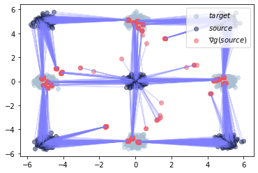
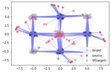
Now, we can plot the corresponding transport from source to target using the gradient of the learning potential \(g\), i.e., \(\nabla g(\text{source})\), or from target to source via the gradient of the learning potential \(f\), i.e., \(\nabla f(\text{target})\).

plot_ot_map(neural_dual, data_source, data_target, inverse=False)

plot_ot_map(neural_dual, data_target, data_source, inverse=True)

We further test, how close the predicted samples are to the sampled data.

First for potential \(g\), transporting source to target samples. Ideally the resulting Sinkhorn distance is close to \(0\).

pred_target = neural_dual.transport(data_source)
print(
    f"Sinkhorn distance between predictions and data samples: {sinkhorn_loss(pred_target, data_target)}"
)

Sinkhorn distance between predictions and data samples: 1.4665195941925049

Then for potential \(f\), transporting target to source samples. Again, the resulting Sinkhorn distance needs to be close to \(0\).

pred_source = neural_dual.transport(data_target, forward=False)
print(
    f"Sinkhorn distance between predictions and data samples: {sinkhorn_loss(pred_source, data_source)}"
)

Sinkhorn distance between predictions and data samples: 6.814591884613037

Besides computing the transport and mapping source to target samples or vice versa, we can also compute the overall distance between new source and target samples.

neural_dual_dist = neural_dual.distance(data_source, data_target)
print(
    f"Neural dual distance between source and target data: {neural_dual_dist}"
)

Neural dual distance between source and target data: 21.16440200805664

Which compares to the primal Sinkhorn distance in the following.

sinkhorn_dist = sinkhorn_loss(data_source, data_target)
print(f"Sinkhorn distance between source and target data: {sinkhorn_dist}")

Sinkhorn distance between source and target data: 21.226734161376953