Sinkhorn Divergence Hessians

Samples two point clouds, computes their Sinkhorn divergence

We show in colab how OTT and JAX can be used to compute automatically the Hessian of the sinkhorn_divergence() w.r.t. the input variables, such as weights a or locations x.

import sys

if "google.colab" in sys.modules:
    !pip install -q git+https://github.com/ott-jax/ott@main

import jax
import jax.numpy as jnp

import matplotlib.pyplot as plt

from ott.geometry import pointcloud
from ott.solvers.linear import implicit_differentiation as implicit_lib
from ott.tools import sinkhorn_divergence

Sample two random point clouds of dimension dim

def sample(n, m, dim):
    rngs = jax.random.split(jax.random.PRNGKey(0), 6)
    x = jax.random.uniform(rngs[0], (n, dim))
    y = jax.random.uniform(rngs[1], (m, dim))
    a = jax.random.uniform(rngs[2], (n,)) + 0.1
    b = jax.random.uniform(rngs[3], (m,)) + 0.1
    a = a / jnp.sum(a)
    b = b / jnp.sum(b)
    return a, x, b, y

a, x, b, y = sample(15, 17, 3)

As usual in JAX, we define a custom loss that outputs the quantity of interest, and is defined using relevant inputs as arguments, i.e. parameters against which we may want to differentiate. We add to a and x the implicit auxiliary flag which will be used to switch between unrolling and implicit differentiation of the Sinkhorn algorithm (see this excellent tutorial for a deep dive on their differences).

The loss outputs the Sinkhorn divergence between two point clouds.

def loss(a, x, implicit):
    return sinkhorn_divergence.sinkhorn_divergence(
        pointcloud.PointCloud,
        x,
        y,  # this part defines geometry
        a=a,
        b=b,  # this sets weights
        sinkhorn_kwargs={
            "implicit_diff": implicit_lib.ImplicitDiff(
                precondition_fun=lambda x: x
            ),
            "use_danskin": False,
        },  # to be used by the Sinkhorn algorithm
    ).divergence

Let’s parse the three lines in the call to sinkhorn_divergence() above:

• The first one defines the point cloud geometry between x and y that will define the cost matrix. Here we could have added details on epsilon regularization (or scheduler), as well as alternative definitions of the cost function (here assumed by default to be squared Euclidean distance). We stick to the default setting.

• The second one sets the respective weight vectors a and b. Those are simply two histograms of size n and m, both sum to 1, in the so-called balanced setting.

• The third one passes on arguments to the three Sinkhorn solvers that will be called, to compare x with y, x with x and y with y with their respective weights a and b. Rather than focusing on the several numerical options available to parameterize Sinkhorn’s behavior, we instruct JAX on how it should differentiate the outputs of the sinkhorn algorithm. The use_danskin flag specifies whether the outputted potentials should be freezed when differentiating. Since we aim for 2nd order differentiation here, we must set this to False (if we wanted to compute gradients, True would have resulted in faster yet almost equivalent computations).

Computing Hessians

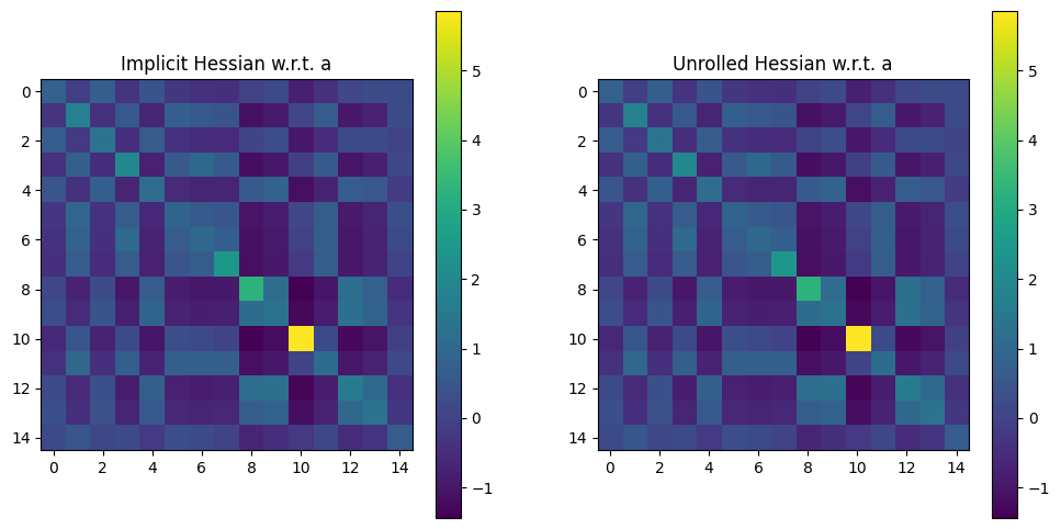
Let’s now plot Hessians of this output w.r.t. either a or x.

• The Hessian w.r.t. a will be a \(n \times n\) matrix, with the convention that a has size \(n\).

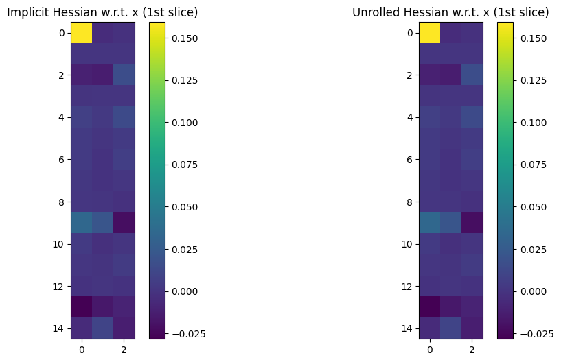
• Because x is itself a matrix of 3D coordinates, the Hessian w.r.t. x will be a 4D tensor of size \(n \times 3 \times n \times 3\).

To plot both Hessians, we loop on arg 0 or 1 of loss, and plot all (or part for x) of those Hessians, to check they match:

for arg in [0, 1]:
    # Compute Hessians using either unrolling or implicit differentiation.
    hess_loss_imp = jax.jit(
        jax.hessian(lambda a, x: loss(a, x, True), argnums=arg)
    )
    print("--- Time: Implicit Hessian w.r.t. " + ("a" if arg == 0 else "x"))
    %timeit _ = hess_loss_imp(a, x).block_until_ready()
    hess_imp = hess_loss_imp(a, x)

    hess_loss_back = jax.jit(
        jax.hessian(lambda a, x: loss(a, x, False), argnums=arg)
    )
    print("--- Time: Unrolled Hessian w.r.t. " + ("a" if arg == 0 else "x"))
    %timeit _ = hess_loss_back(a, x).block_until_ready()
    hess_back = hess_loss_back(a, x)

    # Since we are solving balanced OT problems, Hessians w.r.t. weights are
    # only defined up to the orthogonal space of 1s.
    # For that reason we remove that contribution and check the
    # resulting matrices are equal.
    if arg == 0:
        hess_imp -= jnp.mean(hess_imp, axis=1)[:, None]
        hess_back -= jnp.mean(hess_back, axis=1)[:, None]
    fig, (ax1, ax2) = plt.subplots(1, 2, figsize=(12, 6))
    im = ax1.imshow(hess_imp if arg == 0 else hess_imp[0, 0, :, :])
    ax1.set_title(
        "Implicit Hessian w.r.t. " + ("a" if arg == 0 else "x (1st slice)")
    )
    fig.colorbar(im, ax=ax1)
    im = ax2.imshow(hess_back if arg == 0 else hess_back[0, 0, :, :])
    ax2.set_title(
        "Unrolled Hessian w.r.t. " + ("a" if arg == 0 else "x (1st slice)")
    )
    fig.colorbar(im, ax=ax2)

--- Time: Implicit Hessian w.r.t. a
11.2 ms ± 24.1 µs per loop (mean ± std. dev. of 7 runs, 1 loop each)
--- Time: Unrolled Hessian w.r.t. a
11.2 ms ± 13.5 µs per loop (mean ± std. dev. of 7 runs, 1 loop each)
--- Time: Implicit Hessian w.r.t. x
35.2 ms ± 132 µs per loop (mean ± std. dev. of 7 runs, 1 loop each)
--- Time: Unrolled Hessian w.r.t. x
35.2 ms ± 289 µs per loop (mean ± std. dev. of 7 runs, 1 loop each)