Gromov-Wasserstein

In this tutorial we show how to use a regularised approach [Peyré et al., 2016] to solve the GromovWasserstein (GW) [Mémoli, 2011] problem. The goal of the GW problem is to match points taken within different spaces endowed with their own geometries. At the core of the GW algorithm is the idea of aligning the structures of two geometries, by aligning cost matrices. We illustrate this by calculating the GW distance and the resulting transport matrix between a 2-dimensional and a 3-dimensional shape.

import sys

if "google.colab" in sys.modules:
    !pip install -q git+https://github.com/ott-jax/ott@main

from IPython import display

import jax
import jax.numpy as jnp
import numpy as np

import matplotlib.pyplot as plt
import mpl_toolkits.mplot3d.axes3d as p3
from matplotlib import animation, cm

from ott.geometry import pointcloud
from ott.problems.quadratic import quadratic_problem
from ott.solvers.quadratic import gromov_wasserstein

Matching between spaces with different dimensions

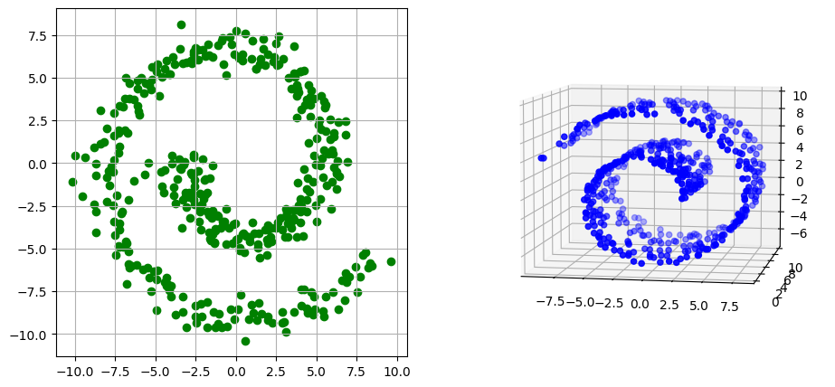
We apply the GromovWasserstein algorithm to a spiral in 2 dimensions and a Swiss roll in 3 dimensions.

To do so, we first generate a spiral and a Swiss roll, and plot them in a 3D space.

# Samples spiral
def sample_spiral(
    n, min_radius, max_radius, key, min_angle=0, max_angle=10, noise=1.0
):
    radius = jnp.linspace(min_radius, max_radius, n)
    angles = jnp.linspace(min_angle, max_angle, n)
    data = []
    noise = jax.random.normal(key, (2, n)) * noise
    for i in range(n):
        x = (radius[i] + noise[0, i]) * jnp.cos(angles[i])
        y = (radius[i] + noise[1, i]) * jnp.sin(angles[i])
        data.append([x, y])
    data = jnp.array(data)
    return data


# Samples Swiss roll
def sample_swiss_roll(
    n, min_radius, max_radius, length, key, min_angle=0, max_angle=10, noise=0.1
):
    spiral = sample_spiral(
        n, min_radius, max_radius, key[0], min_angle, max_angle, noise
    )
    third_axis = jax.random.uniform(key[1], (n, 1)) * length
    swiss_roll = jnp.hstack((spiral[:, 0:1], third_axis, spiral[:, 1:]))
    return swiss_roll


# Plots spiral and Swiss roll
def plot(
    swiss_roll, spiral, colormap_angles_swiss_roll, colormap_angles_spiral
):
    fig = plt.figure(figsize=(11, 5))
    ax = fig.add_subplot(1, 2, 1)
    ax.scatter(spiral[:, 0], spiral[:, 1], c=colormap_angles_spiral)
    ax.grid()
    ax = fig.add_subplot(1, 2, 2, projection="3d")
    ax.view_init(7, -80)
    ax.scatter(
        swiss_roll[:, 0],
        swiss_roll[:, 1],
        swiss_roll[:, 2],
        c=colormap_angles_swiss_roll,
    )
    ax.set_adjustable("box")
    plt.show()

# Data parameters
n_spiral = 400
n_swiss_roll = 500
length = 10
min_radius = 3
max_radius = 10
noise = 0.8
min_angle = 0
max_angle = 9
angle_shift = 3

# Seed
seed = 14
key = jax.random.PRNGKey(seed)
key, *subkey = jax.random.split(key, 4)

spiral = sample_spiral(
    n_spiral,
    min_radius,
    max_radius,
    key=subkey[0],
    min_angle=min_angle + angle_shift,
    max_angle=max_angle + angle_shift,
    noise=noise,
)
swiss_roll = sample_swiss_roll(
    n_swiss_roll,
    min_radius,
    max_radius,
    key=subkey[1:],
    length=length,
    min_angle=min_angle,
    max_angle=max_angle,
)

plot(swiss_roll, spiral, "blue", "green")

We then run OTT’s GromovWasserstein solver to find a matching between the points of each geometry. In this tutorial, we define two PointClouds, but general Geometry objects can be used as well. The loss between the distance matrices of the two pointclouds is by default the squared Euclidean loss.

# apply Gromov-Wasserstein
geom_xx = pointcloud.PointCloud(x=spiral, y=spiral)
geom_yy = pointcloud.PointCloud(x=swiss_roll, y=swiss_roll)
prob = quadratic_problem.QuadraticProblem(geom_xx, geom_yy)

solver = gromov_wasserstein.GromovWasserstein(epsilon=100.0, max_iterations=20)
out = solver(prob)

n_outer_iterations = jnp.sum(out.costs != -1)
has_converged = bool(out.linear_convergence[n_outer_iterations - 1])
print(f"{n_outer_iterations} outer iterations were needed.")
print(f"The last Sinkhorn iteration has converged: {has_converged}")
print(f"The outer loop of Gromov Wasserstein has converged: {out.converged}")
print(f"The final regularised GW cost is: {out.reg_gw_cost:.3f}")

5 outer iterations were needed.
The last Sinkhorn iteration has converged: True
The outer loop of Gromov Wasserstein has converged: True
The final regularised GW cost is: 1183.614

The resulting transport matrix between the two pointclouds is as follows:

transport = out.matrix
fig = plt.figure(figsize=(8, 6))
plt.imshow(transport, cmap="Purples")
plt.xlabel(
    "IDs of samples from the Swiss roll", fontsize=14
)  # IDs are ordered from center to outer part
plt.ylabel(
    "ID of samples from the spiral", fontsize=14
)  # IDs are ordered from center to outer part
plt.colorbar()
plt.show()

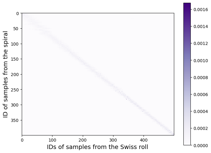
The larger the regularisation parameter epsilon is, the more diffuse the transport matrix becomes, as we can see in the animation below.

# Animates the transport matrix
fig = plt.figure(figsize=(8, 6))
im = plt.imshow(transport, cmap="Purples")
plt.xlabel(
    "IDs of samples from the Swiss roll", fontsize=14
)  # IDs are ordered from center to outer part
plt.ylabel(
    "IDs of samples from the spiral", fontsize=14
)  # IDs are ordered from center to outer part
plt.colorbar()

# Initialization function
def init():
    im.set_data(np.zeros(transport.shape))
    return [im]


# Animation function
def animate(i):
    array = im.get_array()
    geom_xx = pointcloud.PointCloud(x=spiral, y=spiral)
    geom_yy = pointcloud.PointCloud(x=swiss_roll, y=swiss_roll)
    prob = quadratic_problem.QuadraticProblem(geom_xx, geom_yy)

    solver = gromov_wasserstein.GromovWasserstein(epsilon=i, max_iterations=20)

    out = solver(prob)

    im.set_array(out.matrix)
    im.set_clim(0, jnp.max(out.matrix[:]))
    return [im]


# Call the animator
anim = animation.FuncAnimation(
    fig,
    animate,
    init_func=init,
    frames=[70.0, 100.0, 200.0, 500.0, 750.0, 1000.0, 2000.0, 10000.0, 50000.0],
    interval=1500,
    blit=True,
)

html = display.HTML(anim.to_jshtml())
display.display(html)
plt.close()

Once Loop Reflect

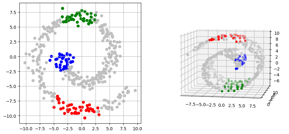
To better understand the correspondance found by the GromovWasserstein solver, we plot in the same color, for each point in the spiral, the point in the Swiss roll it is the most coupled to.

# For each sample from the spiral, we get the most coupled point from the Swiss roll
indices_swiss_roll = jnp.array(np.argmax(transport, axis=1))

# Sets colors to visualise matching of some areas between each shape
# IDs of spiral and Swiss roll are ordered from center to outer part
colors_input_spiral = (
    ["b"] * 40
    + ["silver"] * 160
    + ["g"] * 40
    + ["silver"] * 90
    + ["r"] * 40
    + ["silver"] * 30
)
colors_swiss_roll = np.array(["silver"] * 500)
colors_swiss_roll[indices_swiss_roll[:40]] = "b"
colors_swiss_roll[indices_swiss_roll[200:240]] = "g"
colors_swiss_roll[indices_swiss_roll[330:370]] = "r"

plot(swiss_roll, spiral, colors_swiss_roll, colors_input_spiral)